Submitting
The only files you need to submit are NBody.java and README.txt. If for some reason you create other classes NBody depends on (this is neither necessary nor recommended), submit those as well.
Make sure when you submit, all of the following are present and functional:
Class: NBody
- Method:
public double distance(double, double, double, double) - Method:
public double force(double, double, double) - Method:
public double[][] positions(Scanner, int, int)
Make sure to submit your README in order to receive any credit.
The Equations Behind NBody
###The physics
Here we review the equations governing the motion of the particles according to Newton’s laws of motion and gravitation. Don’t worry if your grounding in physics is a bit rusty or even nonexistent; all of the necessary formulas are included below. We’ll assume for now that the position (px, py) and velocity (vx, vy) of each particle is known. In order to model the dynamics of the system, we must know the net force exerted on each particle.
Pairwise force
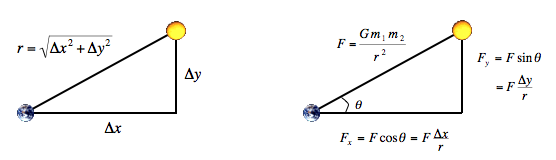
Newton's law of universal gravitation asserts that the strength of the gravitational force between two particles is given by the product of their masses divided by the square of the distance between them, scaled by the gravitational constant G (6.67 × 10⁻¹¹ N m2 / kg2). The pull of one particle towards another acts on the line between them. Since we are using Cartesian coordinates to represent the position of a particle, it is convenient to break up the force into its x and y components (Fx, Fy) as illustrated below.
-
Net force
The principle of superposition says that the net force acting on a particle in the x or y direction is the sum of the pairwise forces acting on the particle in that direction.
Acceleration
Newton's second law of motion postulates that the accelerations in the x and y directions are given by: ax = Fx / m, ay = Fy / m.
###The numerics
We use the leapfrog finite difference approximation scheme to numerically integrate the above equations: this is the basis for most astrophysical simulations of gravitational systems. In the leapfrog scheme, we discretize time, and update the time variable t in increments of the time quantum Δt. We maintain the position (px, py) and velocity (vx, vy) of each particle at each time step. The steps below illustrate how to evolve the positions and velocities of the particles.
- Calculate forces
For each particle:
Calculate the net force (Fx, Fy) at the current time t acting on that particle using Newton's law of gravitation and the principle of superposition. - Update positions, velocities, and acceleration
For each particle:- Calculate its acceleration (ax, ay) at time t using the net force computed in Step 1 and Newton's second law of motion: ax = Fx / m, ay = Fy / m.
- Calculate its new velocity (vx, vy) at the next time step by using the acceleration computed in Step 2a and the velocity from the old time step. Assuming the acceleration remains constant in this interval, the new velocity is (vx + Δt * ax, vy + Δt * ay).
- Calculate its new position (px, py) at time t + Δt by using the velocity computed in Step 2b and its old position at time t. Assuming the velocity remains constant in this interval, the new position is (px + Δt * vx, py + Δt * vy).
- Display update
For each particle
Draw using the position computed in the previous step.
The simulation is more accurate when Δt is very small, but this comes at the price of more computation. The default Δt we use is 25,000, which achieves a reasonable balance.
How To/Suggestions
####Possible Plan
We suggest you implement the algorithm for positions in the following steps.
- Read in the data file planets.txt using the Scanner provided by the method arguments and store the information in six arrays. Use Scanner's
next()method to get the next word,nextInt()to get the next integer, andnextDouble()to get the next real number.</p>Each input file contains the information for a particular universe. The first value is an integer N which represents the number of bodies. The second value is a real number R which represents the radius of the universe. Finally, there are N rows, and each row contains 6 values. The first two values are the x- and y-coordinates of the initial position; the second two values are the x- and y-components of the initial velocity; the next value is the mass; the last value is a String that is the name of an image file used to display the body. As an example, the input file planets.txt contains data for the inner planets of our solar system (in SI units):
5
2.50e11
1.496e11 0.000e00 0.000e00 2.980e04 5.974e24 earth.gif
2.279e11 0.000e00 0.000e00 2.410e04 6.419e23 mars.gif
5.790e10 0.000e00 0.000e00 4.790e04 3.302e23 mercury.gif
0.000e00 0.000e00 0.000e00 0.000e00 1.989e30 sun.gif
1.082e11 0.000e00 0.000e00 3.500e04 4.869e24 venus.gif
Let
px[i], py[i], vx[i], vy[i], andmass[i]be real numbers which store the current position (x and y coordinates), velocity (x and y components), and mass of planet i. Letimage[i]be a string which represents the filename of the image used to display planet i. Keep in mind that some submissions have comments at the end - be sure you read only N lines of input instead of reading until the end of the file.Do not even think of continuing until you have checked that you read in the data correctly. To test, print the information back out using
System.out.println(). -
Plot the background starfield.jpg image. Note that
StdDraw.picture(x, y, file)centers the picture on (x, y). UseStdDraw.setXscale(-R, R)andStdDraw.setYscale(-R, R)to set the boundaries of the simulation. Test that it works. Now, write a loop to plot the N bodies following yourScannercode from step 1. If all goes correctly, you should see the four stationary planets and the sun. Now, go and test it on another data file. This bit of code forms the central basis for your simulation. In the next few steps, you will add code around it and before it to simulate movement and forces. Write a loop to calculate the new velocity and position for each body using
timeStep(This code goes before the plotting code you wrote in the previous step). Since we haven't yet incorporated gravity, assume the acceleration acting on each planet is zero.Add an outer loop to repeat the previous two steps for the duration of
totalTime.To create the illusion of movement, we need to plot each body at its current position using the
StdDraw.picturemethod and display this sequence of snapshots (or frames) in rapid succession. So, after each time step:- draw the background image starfield.jpg,
- redraw all the bodies in their new positions, and
- control the animation speed using
StdDraw.show().
Test your animation. You should now see the four planets moving off the screen in a straight line, with constant velocity. Test it on another data file to be sure.
</li>Now, calculate the net force acting on each body. You will need two additional arrays
fx[i]andfy[i]to store the net force acting on planet i. First, complete thedistance()andforce()methods. Next, withinpositions(), write a loop to initialize all the net forces to 0.0. Then write two nested for loops to calculate the net force exerted by planet j on planet i. (Note: refer to the Equations page for the math.) Add these values to fx[i] and fy[i], but skip the case when i equals j. Once you have these values computed, you can use them to compute the acceleration (instead of assuming it is zero). Test your program on several data files.Your method should finish by returning a 2D array of doubles containing the x and y-positions of the *n* bodies. When you snarf the project, the method
positions()comes with commented instructions on how to return the array in the format the grader expects.When you've finished, you can test if your program works correctly by running it on planets.txt. If you are using the default values time = 10,000,000 and Δt = 25,000, the simulation should show four planets orbiting the sun and stop in this position:
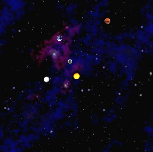
and should produce [this animation](http://www.cs.duke.edu/courses/cps100e/spring10/assign/nbody/nbody-planets.mov).- To make the viewing experience more enjoyable, uncomment the commented line in
start()to play the theme to 2001: A Space Odyssey usingStdAudioand the file 2001.mid. You can also have the program instead play the theme to Superman using superman.mid.
</ol>
- What is the final position of the planets after 1,000,000 seconds with a timestep (i.e. Δt) of 25,000?
- For what values of
timeStep(e.g., Δt > T), does the simulation no longer behave correctly? That is, the planets planets no longer follow their orbits around the Sun. Explain how you arrived at your answer.
Your analysis
In your README.txt, you will answer two questions about the simulation of the bodies described in planets.txt.FAQs
####My computer doesn’t display the animation smoothly. Is there anything I can do?
Use StdDraw.show(30) to turn on the animation mode of standard draw. Call it once at the end of each time step, not after each drawing command.
####Can I combine all the steps from the physics page into one large for loop?
No! This will simultaneously screw up the physics and make your code harder to understand and debug.
####I draw the planets, but nothing appears on the screen. Why?
Use StdDraw.setXscale() and StdDraw.setYscale() to change the coordinate system to use the physics coordinates instead of the unit box.
####My planets don’t move.
Make sure that you are using a large enough value of Δt (we specify 25000, but you might want a smaller one when debugging).
####My planets move, but leave images of themselves behind.
Make sure you redraw starfield.jpg once per loop before drawing all your planets, instead of just once for the entire simulation. If your simulation begins to lag, you may also want to clear all of the images on each iteration.
####My planets repel each other instead of attracting each other.
Make sure that you get the sign right when you apply Newton’s law of gravitation: (x[j] - x[i]) vs. (x[i] - x[j]). Note that Δx and Δy can be positive or negative so do not use Math.abs(). Do not consider changing the universal gravitational constant G to patch your code!
####How should I compute x2?
The simplest way is x*x. In Java, the ^ operator means XOR or “exclusive or” rather than exponentation.
####How should I compute the square root of x?
Use Math.sqrt or Math.pow. The return value of Math.pow(a, b) is ab.
####What is Δx?
It’s the change in x-coordinate between two bodies (not between a body at time t and at time t + Δt).
####When I compile NBody.java, it says “cannot resolve symbol StdDraw.”
Make sure that you import princeton.* and add princeton.jar to your library build path.
####When should my planets move?
Since we are doing a leapfrog calculation, you should calculate every net force experienced by the objects in the system before you allow them to move. A leapfrog calculation can be thought of in terms of a snapshot: you take a snapshot of the system with the planets held in place, calculate the force, acceleration, velocity, and position, then you allow the planets to move for the amount of time specified by timeStep. This repeats until the simulation terminates (i.e. you reach totalTime)
####I’m a physicist. Why should I use the leapfrog method instead of the formula I derived in high school?
The leapfrog method is more stable for integrating Hamiltonian systems than conventional numerical methods like Euler’s method or Runge-Kutta. The leapfrog method is symplectic, which means it preserves properties specific to Hamiltonian systems (conservation of linear and angular momentum, time-reversibility, and conservation of energy of the discrete Hamiltonian). In contrast, ordinary numerical methods become dissipative and exhibit qualitatively different long-term behavior. For example, the earth would slowly spiral into (or away from) the sun. For these reasons, symplectic methods are extremely popular for N-body calculations in practice. You asked!
Grading
Testing your code
We will be grading your project by calling the method positions on test cases, and seeing if your output matches the expected output. You can test whether positions is producing the correct array by inserting the following code into your main method:
double[][] test = myNBody.positions(new Scanner(new File("data/planets.txt")), 100000, 25000);
for(int i = 0; i < test.length; i++) {
    for(int j = 0; j < test[i].length; j++) {
        System.out.print(test[i][j]+" ");
    }
    System.out.println();
}
This should output the following in console:
1.4956294976553436E11 2.9798154903465266E9
2.2788403506932733E11 2.409957795285363E9
5.765266792231076E10 4.784879361438483E9
330.8671434437699 2.820200096518896
1.0812917648253027E11 3.499427153160241E9
Automated Tests
Below is a list of aspects of your code the automated tests will check. Your code will still be checked by a TA, and passing all these tests does not guarantee a perfect grade.
- Does the
forcemethod return the right output? - Does the
distancemethod return the right output? - Does the
positionsmethod return the right output? - Does the
positionsmethod process files with comments correctly? - Does the
positionsmethod use.next(),.nextInt(), and.nextDouble()to process files? - Does the
positionsmethod process universes with only one or two bodies correctly? - Does the
positionsmethod handle odd time steps correctly/is the timing for loop written correctly? (e.g. running withtimeStep= 25000, and 25001 should both update positions twice usingtotalTime= 50000, buttimeStep= 24999 should update thrice) - Does the
positionsmethod process universes with 100+ bodies? - Does the
positionsmethod callStdDraw.show()the correct number of times?
Point Breakdown
This assignment is worth 25 points.
- 85% algorithmic/correctness: for the correctness of your implementation of NBody (based largely on whether it passes our automated tests).
- 5% engineering: for the structure and style of your NBody implementation. Does your solution decompose the problem appropriately? Is your code formatted appropriately?
- 10% analysis: for your README.txt and answers to the analysis questions.
NBody Simulation
##NBody - Overview
This assignment and writeup was originally developed by Kevin Wayne and Robert Sedgewick at Princeton University.
You can download the skeleton code from the snarf site using Ambient, or the equivalent .jar to import from here. Submit the assignment to the nbody folder. You should only need to submit your README and the NBody.java class. Make sure you submit the latter within the src folder.
You can also view/download the NBody class here:
We suggest you read the “Equations Behind NBody” and “Suggestions/How To” sections before writing any code.
Here is a printer friendly version of this assignment.
###Background
In 1687 Sir Isaac Newton formulated the principles governing the the motion of two particles under the influence of their mutual gravitational attraction in his famous Principia[1]. However, Newton was unable to solve the problem for three particles. Indeed, in general, systems of three or more particles can only be solved numerically. The N-Body problem is a reoccuring problem in many disciplines - from Biology and Biochemistry to Physics and Astronomy to Hydrology and Aerodynamics[2].
In this assignment, you will write a program to simulate the motion of N particles, mutually affected by gravitational forces, and animate the results. Such methods are widely used in cosmology, semiconductors, and fluid dynamics to study complex physical systems. Scientists also apply the same techniques to other pairwise interactions including Coulombic, Biot-Savart, and van der Waals.
###References [1] Newton, Isaac. Philosophiae naturalis principia mathematica. 1713.
[2] Lubomir Ivanov, “The N-Body problem throughout the Computer Science Curriculum”